Quickstart
![]()
We are glad this package caught your attention, so let’s try to briefly showcase its power.
Data
In this tutorial, we will use a historical Rossmann sales dataset that we load via the hcrystalball.utils.get_sales_data function.
A description of the dataset and available columns is given in the docstring.
[1]:
import pandas as pd
import matplotlib.pyplot as plt
plt.style.use('seaborn')
plt.rcParams['figure.figsize'] = [12, 6]
[2]:
from hcrystalball.utils import get_sales_data

df = get_sales_data(n_dates=100,
                    n_assortments=2,
                    n_states=2,
                    n_stores=2)
[3]:
df
[3]:
| Store | Sales | Open | Promo | SchoolHoliday | StoreType | Assortment | Promo2 | State | HolidayCode | |
|---|---|---|---|---|---|---|---|---|---|---|
| Date | ||||||||||
| 2015-04-23 | 817 | 17520 | True | False | False | a | a | False | BE | DE-BE |
| 2015-04-23 | 251 | 16573 | True | False | False | a | c | False | NW | DE-NW |
| 2015-04-23 | 335 | 11189 | True | False | False | b | a | True | NW | DE-NW |
| 2015-04-23 | 380 | 10761 | True | False | False | a | a | True | NW | DE-NW |
| 2015-04-23 | 788 | 15793 | True | False | False | a | c | False | BE | DE-BE |
| ... | ... | ... | ... | ... | ... | ... | ... | ... | ... | ... |
| 2015-07-31 | 523 | 15349 | True | True | True | c | c | False | BE | DE-BE |
| 2015-07-31 | 513 | 19959 | True | True | True | a | a | False | BE | DE-BE |
| 2015-07-31 | 380 | 17133 | True | True | True | a | a | True | NW | DE-NW |
| 2015-07-31 | 335 | 17867 | True | True | True | b | a | True | NW | DE-NW |
| 2015-07-31 | 251 | 22205 | True | True | True | a | c | False | NW | DE-NW |
800 rows × 10 columns
Define search space
Next step is to define ModelSelector for which frequency the data will be resampled to, how many steps ahead the forecast should run, and optionally define column, which contains ISO code of country/region to take holiday information for given days
Once done, creating grid search with possible exogenous columns and extending it with custom models
[4]:
from hcrystalball.model_selection import ModelSelector

ms = ModelSelector(horizon=10,
                   frequency='D',
                   country_code_column='HolidayCode',
                  )

ms.create_gridsearch(sklearn_models=True,
                    n_splits = 2,
                    between_split_lag=None,
                    sklearn_models_optimize_for_horizon=False,
                    autosarimax_models=False,
                    prophet_models=False,
                    tbats_models=False,
                    exp_smooth_models=False,
                    average_ensembles=False,
                    stacking_ensembles=False,
                    exog_cols=['Open','Promo','SchoolHoliday','Promo2'],
#                     holidays_days_before=2,
#                     holidays_days_after=1,
#                     holidays_bridge_days=True,
                    )
[5]:
from hcrystalball.wrappers import get_sklearn_wrapper
from sklearn.linear_model import LinearRegression

ms.add_model_to_gridsearch(get_sklearn_wrapper(LinearRegression))
Run model selection
By default the run will partition data by partition_columns and do for loop over all partitions.
If you have a problem, that make parallelization overhead worth trying, you can also use parallel_columns - subset of partition_columns over which the parallel run (using prefect) will be started.
If expecting the run to take long, it might be good to directly store results. Here output_path and persist_ methods might come convenient
[6]:
# from prefect.engine.executors import LocalDaskExecutor
ms.select_model(df=df,
                target_col_name='Sales',
                partition_columns=['Assortment', 'State','Store'],
#                 parallel_over_columns=['Assortment'],
#                 persist_model_selector_results=False,
#                 output_path='my_results',
#                 executor = LocalDaskExecutor(),
               )
Look at the results
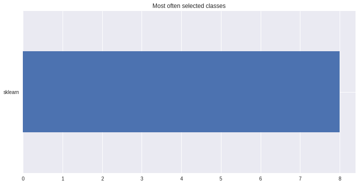
Naturaly we are interested in which models were chosen, so that we can strip our parameter grid from the ones, which were failing and extend with more sophisticated models from most selected classes
[7]:
ms.plot_best_wrapper_classes();
[7]:
<matplotlib.axes._subplots.AxesSubplot at 0x7fb145fda310>
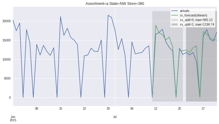
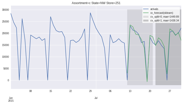
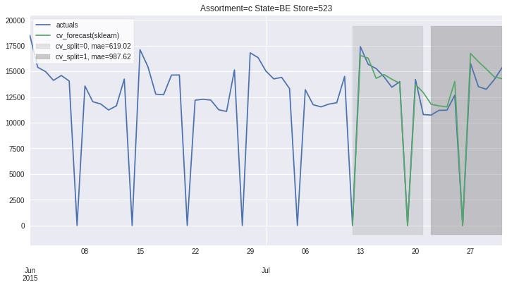
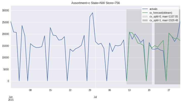
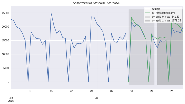
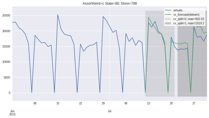
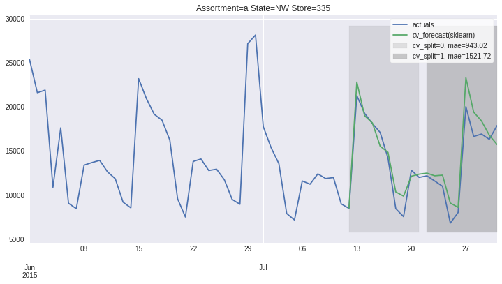
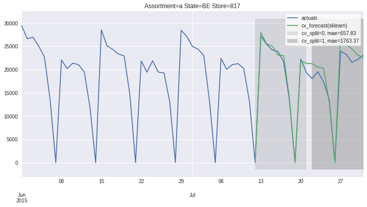
There also exists convenient method to plot the results over all (or subset of) the data partitions to see how well our model fitted the data during cross validation
[8]:
ms.plot_results(plot_from='2015-06-01');
[8]:
[<matplotlib.axes._subplots.AxesSubplot at 0x7fb143bfead0>,
 <matplotlib.axes._subplots.AxesSubplot at 0x7fb15661e350>,
 <matplotlib.axes._subplots.AxesSubplot at 0x7fb143a25350>,
 <matplotlib.axes._subplots.AxesSubplot at 0x7fb143981890>,
 <matplotlib.axes._subplots.AxesSubplot at 0x7fb143862550>,
 <matplotlib.axes._subplots.AxesSubplot at 0x7fb143862450>,
 <matplotlib.axes._subplots.AxesSubplot at 0x7fb1437c7490>,
 <matplotlib.axes._subplots.AxesSubplot at 0x7fb14360fad0>]


Accessing 1 Time-Series
To get to more information, it is advisable to go from all partitions level (ModelSelector) to single partition level (ModelSelectorResult).
ModelSelector stores results as a list of ModelSelectorResult objects in self.results. Here we provide rich __repr__ that hints on what information are available.
Another way to get the ModelSelectorResult is to use ModelSelector.get_result_for_partition that ensures the same results also when loading the stored results. Here the list access method fails (ModelSelector.results[0]), because each ModelSelectorResults is stored with partition_hash name and later load ingests these files in alphabetical order.
Accessing training data to see what is behind the model, cv_results to check the fitting time or how big margin my best model had over the second best one or access model definition and explore its parameters are all handy things that we found useful
[9]:
ms.results[0]
[9]:
ModelSelectorResult
-------------------
  best_model_name: sklearn
  frequency: D
  horizon: 10

  country_code_column: HolidayCode

  partition: {'Assortment': 'a', 'State': 'NW', 'Store': 335}
  partition_hash: 0d8965bc23395b49a81bdc3834bc15fb

  df_plot: DataFrame (100, 6) suited for plotting cv results with .plot()
  X_train: DataFrame (100, 6) with training feature values
  y_train: DataFrame (100,) with training target values
  cv_results: DataFrame (19, 16) with gridsearch cv info
  best_model_cv_results: Series with gridsearch cv info
  cv_data: DataFrame (20, 21) with models predictions, split and true target values
  best_model_cv_data: DataFrame (20, 3) with model predictions, split and true target values

  model_reprs: Dict of model_hash and model_reprs
  best_model_hash: c8e63205e1e0fbcd8e2df5bc3eea96a7
  best_model: Pipeline(memory=None,
         steps=[('exog_passthrough',
                 TSColumnTransformer(n_jobs=None, remainder='drop',
                                     sparse_threshold=0.3,
                                     transformer_weights=None,
                                     transformers=[('raw_cols', 'passthrough',
                                                    ['Open', 'Promo',
                                                     'SchoolHoliday', 'Promo2',
                                                     'HolidayCode'])],
                                     verbose=False)),
                ('holiday',
                 Pipeline(memory=None,
                          steps=[('holiday_HolidayCode',
                                  HolidayTransformer(bridge_days=...
                                                 max_depth=6,
                                                 max_features='auto',
                                                 max_leaf_nodes=None,
                                                 max_samples=None,
                                                 min_impurity_decrease=0.0,
                                                 min_impurity_split=None,
                                                 min_samples_leaf=1,
                                                 min_samples_split=2,
                                                 min_weight_fraction_leaf=0.0,
                                                 n_estimators=100, n_jobs=None,
                                                 name='sklearn',
                                                 oob_score=False,
                                                 optimize_for_horizon=False,
                                                 random_state=None, verbose=0,
                                                 warm_start=False))],
                          verbose=False))],
         verbose=False)
-------------------
[10]:
res = ms.get_result_for_partition(partition=ms.results[0].partition)
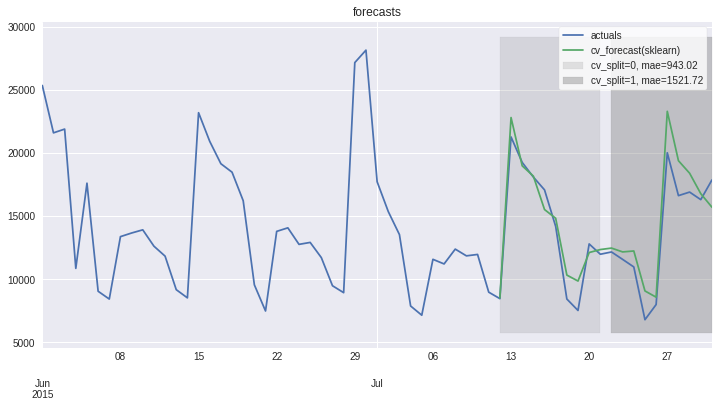
Plotting results and errors for 1 time series
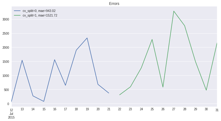
On this level we can also access the forecast plots - one that we already know with cv_forecasts and one that gives us only errors
[11]:
res.plot_result(plot_from = '2015-06-01', title='forecasts');
[11]:
<matplotlib.axes._subplots.AxesSubplot at 0x7fb141b8c090>
[12]:
res.plot_error(title='Errors');
[12]:
cv_split_str
cv_split=0, mae=943.02     AxesSubplot(0.125,0.125;0.775x0.755)
cv_split=1, mae=1521.72    AxesSubplot(0.125,0.125;0.775x0.755)
Name: error, dtype: object
Persist and load
To enable later usage of our found results, there are plenty of methods that can help storing and loading the results of model selection in a uniform way.
Some methods and functions persits/load the whole objects (load_model_selector, load_model_selector_result), while some provide direct access to the part we might only care if we run in production and have space limitations (load_best_model, load_partition, …)
[13]:
from hcrystalball.model_selection import load_model_selector
from hcrystalball.model_selection import load_model_selector_result
from hcrystalball.model_selection import load_best_model

res.persist(path='tmp')
res = load_model_selector_result(path='tmp',partition_label=ms.results[0].partition)

ms.persist_results(folder_path='tmp/results')
ms = load_model_selector(folder_path='tmp/results')
[14]:
ms = load_model_selector(folder_path='tmp/results')
[15]:
ms.plot_results(plot_from='2015-06-01');
[15]:
[<matplotlib.axes._subplots.AxesSubplot at 0x7fb143c86a10>,
 <matplotlib.axes._subplots.AxesSubplot at 0x7fb143c56050>,
 <matplotlib.axes._subplots.AxesSubplot at 0x7fb143c69c50>,
 <matplotlib.axes._subplots.AxesSubplot at 0x7fb1417cde90>,
 <matplotlib.axes._subplots.AxesSubplot at 0x7fb14173b090>,
 <matplotlib.axes._subplots.AxesSubplot at 0x7fb14173b350>,
 <matplotlib.axes._subplots.AxesSubplot at 0x7fb14160ec50>,
 <matplotlib.axes._subplots.AxesSubplot at 0x7fb1414f2210>]


[16]:
# cleanup
import shutil
try:
    shutil.rmtree('tmp')
except:
    pass