Advanced Large Scale learning with ModelSelector
Very often we have many different products, regions, countries, shops…for which we need to delivery forecast. This can be easily done with ModelSelector
[1]:
import pandas as pd
import matplotlib.pyplot as plt
plt.style.use('seaborn')
plt.rcParams['figure.figsize'] = [12, 6]
[2]:
from hcrystalball.model_selection import ModelSelector
from hcrystalball.utils import get_sales_data
from hcrystalball.wrappers import get_sklearn_wrapper
from sklearn.linear_model import LinearRegression
from sklearn.ensemble import RandomForestRegressor
Get Dummy Data
[3]:
df = get_sales_data(n_dates=365*2,
                    n_assortments=2,
                    n_states=2,
                    n_stores=2)
[4]:
df.head()
[4]:
| Store | Sales | Open | Promo | SchoolHoliday | StoreType | Assortment | Promo2 | State | HolidayCode | |
|---|---|---|---|---|---|---|---|---|---|---|
| Date | ||||||||||
| 2013-08-01 | 817 | 25013 | True | True | True | a | a | False | BE | DE-BE |
| 2013-08-01 | 251 | 18633 | True | True | True | a | c | False | NW | DE-NW |
| 2013-08-01 | 335 | 16324 | True | True | True | b | a | True | NW | DE-NW |
| 2013-08-01 | 380 | 15092 | True | True | True | a | a | True | NW | DE-NW |
| 2013-08-01 | 788 | 19788 | True | True | True | a | c | False | BE | DE-BE |
Get predefined sklearn models, holidays and exogenous variables
Here for the sake of time, we will use the advantage of the create_gridsearch method for cv splits, default scorer etc. and just extend empty grid with two models
[5]:
ms = ModelSelector(frequency='D', horizon=10, country_code_column='HolidayCode')
[6]:
# see full default parameter grid in hands on exercise
ms.create_gridsearch(
    n_splits=2,
    between_split_lag=5, # create overlapping cv_splits
    sklearn_models=False,
    sklearn_models_optimize_for_horizon=False,
    autosarimax_models=False,
    prophet_models=False,
    tbats_models=False,
    exp_smooth_models=False,
    average_ensembles=False,
    stacking_ensembles=False,
    exog_cols=['Open','Promo','SchoolHoliday','Promo2'],
)
[7]:
ms.add_model_to_gridsearch(get_sklearn_wrapper(LinearRegression))
ms.add_model_to_gridsearch(get_sklearn_wrapper(RandomForestRegressor))
Run model selection with partitions
This can be done within classical for loop that enables you to see progress bar, or within parallelized prefect flow in case you would define parallel_over_columns, which must be subset of partition_columns and optionally add executor to point to your running dask cluster. Default uses LocalExecutor, you might also try LocalDaskExecutor, that prefect will spin up for you DaskExecutor if you have one already running and you want to connect to it.
[8]:
df
[8]:
| Store | Sales | Open | Promo | SchoolHoliday | StoreType | Assortment | Promo2 | State | HolidayCode | |
|---|---|---|---|---|---|---|---|---|---|---|
| Date | ||||||||||
| 2013-08-01 | 817 | 25013 | True | True | True | a | a | False | BE | DE-BE |
| 2013-08-01 | 251 | 18633 | True | True | True | a | c | False | NW | DE-NW |
| 2013-08-01 | 335 | 16324 | True | True | True | b | a | True | NW | DE-NW |
| 2013-08-01 | 380 | 15092 | True | True | True | a | a | True | NW | DE-NW |
| 2013-08-01 | 788 | 19788 | True | True | True | a | c | False | BE | DE-BE |
| ... | ... | ... | ... | ... | ... | ... | ... | ... | ... | ... |
| 2015-07-31 | 523 | 15349 | True | True | True | c | c | False | BE | DE-BE |
| 2015-07-31 | 513 | 19959 | True | True | True | a | a | False | BE | DE-BE |
| 2015-07-31 | 380 | 17133 | True | True | True | a | a | True | NW | DE-NW |
| 2015-07-31 | 335 | 17867 | True | True | True | b | a | True | NW | DE-NW |
| 2015-07-31 | 251 | 22205 | True | True | True | a | c | False | NW | DE-NW |
5840 rows × 10 columns
[9]:
# from prefect.engine.executors import LocalDaskExecutor
ms.select_model(df=df,
                target_col_name='Sales',
                partition_columns=['Assortment', 'State', 'Store'],
#                 parallel_over_columns=['Assortment'],
#                 executor = LocalDaskExecutor(),
               )
[10]:
ms.get_partitions(as_dataframe=True)
[10]:
| State | Assortment | Store | |
|---|---|---|---|
| 0 | BE | a | 513 |
| 1 | BE | a | 817 |
| 2 | BE | c | 523 |
| 3 | BE | c | 788 |
| 4 | NW | a | 335 |
| 5 | NW | a | 380 |
| 6 | NW | c | 251 |
| 7 | NW | c | 756 |
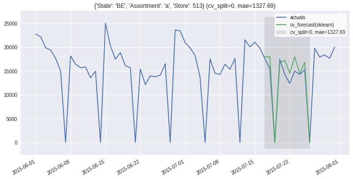
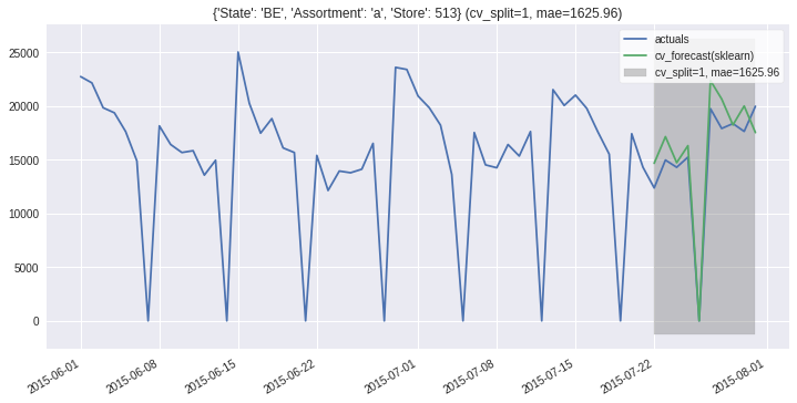
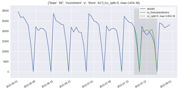
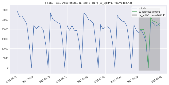
[11]:
ms.plot_results(partitions=ms.partitions[:2], plot_from='2015-06');