Advanced Prophet Usage
You can scan through prophet docs and find many options how to tweak your model. Some of that functionality is moved to initialization stage to be compatible with Sklearn API. We will showcase the parts that were moved to initialization, but you can also look for other model parameters that could help fine-tuning your model
[1]:
import pandas as pd
import numpy as np
import matplotlib.pyplot as plt
plt.style.use('seaborn')
plt.rcParams['figure.figsize'] = [12, 6]
[2]:
from hcrystalball.utils import generate_tsdata
X, y = generate_tsdata(n_dates=365*2)
[3]:
from hcrystalball.wrappers import ProphetWrapper
[4]:
ProphetWrapper?
Advanced Holidays
For holidays, we are able to define instead of single boolean attribute distribution around given day. We define lower_window, upper_window and prior_scales
[5]:
extra_holidays = {
    'Christmas Day':{'lower_window': -2, 'upper_window':2, 'prior_scale': 20},
#     'Good Friday':{'lower_window': -1, 'upper_window':1, 'prior_scale': 30}
}
Unusual Seasonalities
[6]:
extra_seasonalities = [
    {
        'name':'bi-weekly',
        'period': 14.,
        'fourier_order': 5,
        'prior_scale': 10.0,
        'mode': None
    },
    {
        'name':'bi-yearly',
        'period': 365*2.,
        'fourier_order': 5,
        'prior_scale': 5.0,
        'mode': None
    },
]
Exogenous Variables
[7]:
from sklearn.pipeline import Pipeline
from hcrystalball.feature_extraction import HolidayTransformer
[8]:
extra_regressors = ['trend_line']
X['trend_line'] = np.arange(len(X))
[9]:
prophet = ProphetWrapper(
    name='prophet',
)
prophet_extra = ProphetWrapper(
    extra_holidays=extra_holidays,
    extra_seasonalities=extra_seasonalities,
    extra_regressors=extra_regressors,
    name='prophet_extra',
)
[10]:
pipeline = Pipeline([
    ('holidays_de', HolidayTransformer(country_code = 'DE')),
    ('model', prophet)
])
pipeline_extra = Pipeline([
    ('holidays_de', HolidayTransformer(country_code = 'DE')),
    ('model', prophet_extra)
])
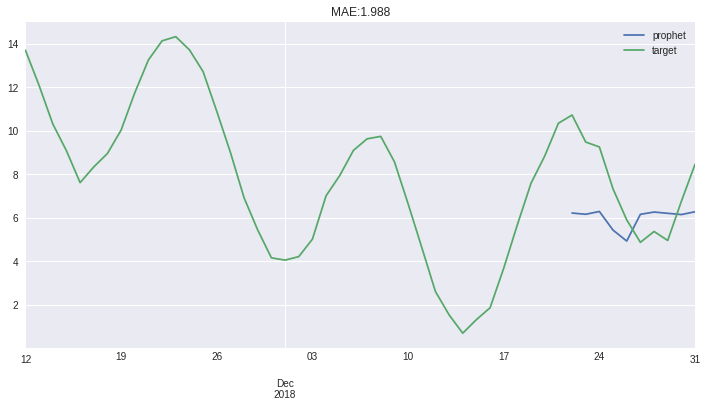
[11]:
prds = (pipeline.fit(X[:-10], y[:-10])
         .predict(X[-10:])
         .merge(y, left_index=True, right_index=True, how='outer')
         .tail(50))

prds.plot(title=f"MAE:{(prds['target']-prds['prophet']).abs().mean().round(3)}");
[11]:
<AxesSubplot:title={'center':'MAE:1.988'}>
[12]:
prds_extra = (pipeline_extra.fit(X[:-10], y[:-10])
         .predict(X[-10:])
         .merge(y, left_index=True, right_index=True, how='outer')
         .tail(50))

prds_extra.plot(title=f"MAE:{(prds_extra['target']-prds_extra['prophet_extra']).abs().mean().round(3)}");
[12]:
<AxesSubplot:title={'center':'MAE:3.716'}>
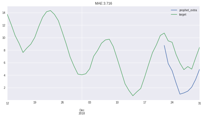
Compared to non-tweaked model, we are able to better catch the series dynamics, but don’t win in MAE against roughly average predictions
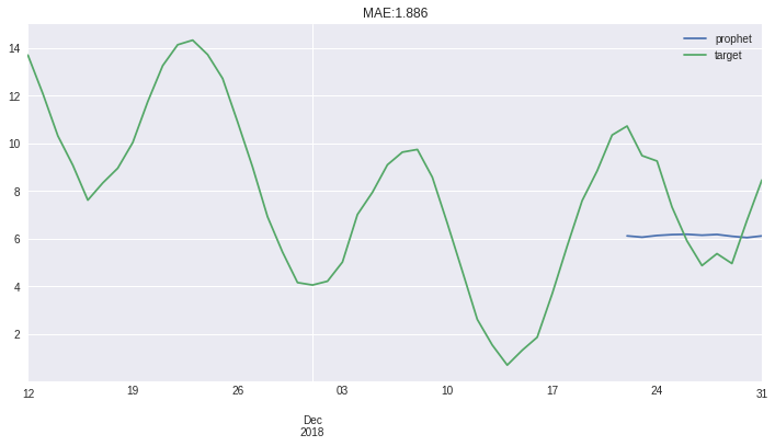
[13]:
prds = (ProphetWrapper().fit(X[:-10], y[:-10])
                 .predict(X[-10:])
                 .merge(y, left_index=True, right_index=True, how='outer')
                 .tail(50)
)
prds.plot(title=f"MAE:{(prds['target']-prds['prophet']).abs().mean().round(3)}");
[13]:
<AxesSubplot:title={'center':'MAE:1.886'}>
Full Prophet Output
If you need, you can also pass full_prophet_output and get rich predict output
[14]:
(ProphetWrapper(full_prophet_output=True, conf_int=True)
     .fit(X[:-10], y[:-10])
     .predict(X[-10:])
)
[14]:
| trend | prophet_lower | prophet_upper | trend_lower | trend_upper | additive_terms | additive_terms_lower | additive_terms_upper | weekly | weekly_lower | weekly_upper | multiplicative_terms | multiplicative_terms_lower | multiplicative_terms_upper | prophet | |
|---|---|---|---|---|---|---|---|---|---|---|---|---|---|---|---|
| 2018-12-22 | 6.151973 | 1.038690 | 11.545119 | 6.151973 | 6.151973 | -0.031628 | -0.031628 | -0.031628 | -0.031628 | -0.031628 | -0.031628 | 0.0 | 0.0 | 0.0 | 6.120344 |
| 2018-12-23 | 6.149407 | 1.087590 | 11.920487 | 6.149407 | 6.149407 | -0.084270 | -0.084270 | -0.084270 | -0.084270 | -0.084270 | -0.084270 | 0.0 | 0.0 | 0.0 | 6.065137 |
| 2018-12-24 | 6.146841 | 0.857559 | 11.610195 | 6.146841 | 6.146841 | -0.010959 | -0.010959 | -0.010959 | -0.010959 | -0.010959 | -0.010959 | 0.0 | 0.0 | 0.0 | 6.135883 |
| 2018-12-25 | 6.144276 | 0.756582 | 11.534445 | 6.144276 | 6.144276 | 0.029113 | 0.029113 | 0.029113 | 0.029113 | 0.029113 | 0.029113 | 0.0 | 0.0 | 0.0 | 6.173389 |
| 2018-12-26 | 6.141710 | 0.779932 | 11.676427 | 6.141710 | 6.141710 | 0.045507 | 0.045507 | 0.045507 | 0.045507 | 0.045507 | 0.045507 | 0.0 | 0.0 | 0.0 | 6.187217 |
| 2018-12-27 | 6.139144 | 0.594331 | 11.537535 | 6.139144 | 6.139144 | 0.009433 | 0.009433 | 0.009433 | 0.009433 | 0.009433 | 0.009433 | 0.0 | 0.0 | 0.0 | 6.148578 |
| 2018-12-28 | 6.136579 | 0.937165 | 11.405285 | 6.136578 | 6.136590 | 0.042803 | 0.042803 | 0.042803 | 0.042803 | 0.042803 | 0.042803 | 0.0 | 0.0 | 0.0 | 6.179382 |
| 2018-12-29 | 6.134013 | 0.000953 | 11.264760 | 6.133966 | 6.134073 | -0.031628 | -0.031628 | -0.031628 | -0.031628 | -0.031628 | -0.031628 | 0.0 | 0.0 | 0.0 | 6.102385 |
| 2018-12-30 | 6.131447 | 0.426198 | 11.261615 | 6.131264 | 6.131579 | -0.084270 | -0.084270 | -0.084270 | -0.084270 | -0.084270 | -0.084270 | 0.0 | 0.0 | 0.0 | 6.047178 |
| 2018-12-31 | 6.128882 | 0.899522 | 11.434409 | 6.128583 | 6.129082 | -0.010959 | -0.010959 | -0.010959 | -0.010959 | -0.010959 | -0.010959 | 0.0 | 0.0 | 0.0 | 6.117923 |