Inspecting ModelSelectorResult
When we go down from multiple time-series to single time-series, the best way how to get access to all relevant information to use/access ModelSelectorResult objects
[1]:
import pandas as pd
import matplotlib.pyplot as plt
plt.style.use('seaborn')
plt.rcParams['figure.figsize'] = [12, 6]
[2]:
from hcrystalball.model_selection import ModelSelector
from hcrystalball.utils import get_sales_data
from hcrystalball.wrappers import get_sklearn_wrapper
from sklearn.linear_model import LinearRegression
from sklearn.ensemble import RandomForestRegressor
[3]:
df = get_sales_data(n_dates=365*2,
                    n_assortments=1,
                    n_states=1,
                    n_stores=2)
df.head()
[3]:
| Store | Sales | Open | Promo | SchoolHoliday | StoreType | Assortment | Promo2 | State | HolidayCode | |
|---|---|---|---|---|---|---|---|---|---|---|
| Date | ||||||||||
| 2013-08-01 | 817 | 25013 | True | True | True | a | a | False | BE | DE-BE |
| 2013-08-01 | 513 | 22514 | True | True | True | a | a | False | BE | DE-BE |
| 2013-08-02 | 513 | 19330 | True | True | True | a | a | False | BE | DE-BE |
| 2013-08-02 | 817 | 22870 | True | True | True | a | a | False | BE | DE-BE |
| 2013-08-03 | 513 | 16633 | True | False | False | a | a | False | BE | DE-BE |
[4]:
# let's start simple
df_minimal = df[['Sales']]
[5]:
ms_minimal = ModelSelector(frequency='D', horizon=10)
[6]:
ms_minimal.create_gridsearch(
    n_splits=2,
    between_split_lag=None,
    sklearn_models=False,
    sklearn_models_optimize_for_horizon=False,
    autosarimax_models=False,
    prophet_models=False,
    tbats_models=False,
    exp_smooth_models=False,
    average_ensembles=False,
    stacking_ensembles=False)
[7]:
ms_minimal.add_model_to_gridsearch(get_sklearn_wrapper(LinearRegression, hcb_verbose=False))
ms_minimal.add_model_to_gridsearch(get_sklearn_wrapper(RandomForestRegressor, random_state=42, hcb_verbose=False))
[8]:
ms_minimal.select_model(df=df_minimal, target_col_name='Sales')
Ways to access ModelSelectorResult
There are three ways how you can get to single time-series result level.
First is over
.results[i], which is fast, but does not ensure, that results are loaded in the same order as when they were created (reason for that is hash used in the name of each result, that are later read in alphabetic order)Second and third uses
.get_result_for_partition()throughdictbased partitionForth does that using
partition_hash(also in results file name if persisted)
[9]:
result = ms_minimal.results[0]
result = ms_minimal.get_result_for_partition({'no_partition_label': ''})
result = ms_minimal.get_result_for_partition(ms_minimal.partitions[0])
result = ms_minimal.get_result_for_partition('fb452abd91f5c3bcb8afa4162c6452c2')
ModelSelectorResult is rich
As you can see below, we try to store all relevant information to enable easy access to data, that is otherwise very lenghty.
[10]:
result
[10]:
ModelSelectorResult
-------------------
  best_model_name: sklearn
  frequency: D
  horizon: 10

  country_code_column: None

  partition: {'no_partition_label': ''}
  partition_hash: fb452abd91f5c3bcb8afa4162c6452c2

  df_plot: DataFrame (730, 6) suited for plotting cv results with .plot()
  X_train: DataFrame (730, 0) with training feature values
  y_train: DataFrame (730,) with training target values
  cv_results: DataFrame (2, 11) with gridsearch cv info
  best_model_cv_results: Series with gridsearch cv info
  cv_data: DataFrame (20, 4) with models predictions, split and true target values
  best_model_cv_data: DataFrame (20, 3) with model predictions, split and true target values

  model_reprs: Dict of model_hash and model_reprs
  best_model_hash: 53ec261970542c03a3b0a54fc6af214d
  best_model: Pipeline(memory=None,
         steps=[('exog_passthrough', 'passthrough'), ('holiday', 'passthrough'),
                ('model',
                 SklearnWrapper(bootstrap=True, ccp_alpha=0.0,
                                clip_predictions_lower=None,
                                clip_predictions_upper=None, criterion='mse',
                                fit_params=None, hcb_verbose=False, lags=3,
                                max_depth=None, max_features='auto',
                                max_leaf_nodes=None, max_samples=None,
                                min_impurity_decrease=0.0,
                                min_impurity_split=None, min_samples_leaf=1,
                                min_samples_split=2,
                                min_weight_fraction_leaf=0.0, n_estimators=100,
                                n_jobs=None, name='sklearn', oob_score=False,
                                optimize_for_horizon=False, random_state=42,
                                verbose=0, warm_start=False))],
         verbose=False)
-------------------
Traning data
[11]:
result.X_train
[11]:
| Date |
|---|
| 2013-08-01 |
| 2013-08-02 |
| 2013-08-03 |
| 2013-08-04 |
| 2013-08-05 |
| ... |
| 2015-07-27 |
| 2015-07-28 |
| 2015-07-29 |
| 2015-07-30 |
| 2015-07-31 |
730 rows × 0 columns
[12]:
result.y_train
[12]:
Date
2013-08-01    47527
2013-08-02    42200
2013-08-03    30370
2013-08-04        0
2013-08-05    42239
              ...
2015-07-27    43671
2015-07-28    41142
2015-07-29    39906
2015-07-30    39800
2015-07-31    43052
Freq: D, Name: Sales, Length: 730, dtype: int64
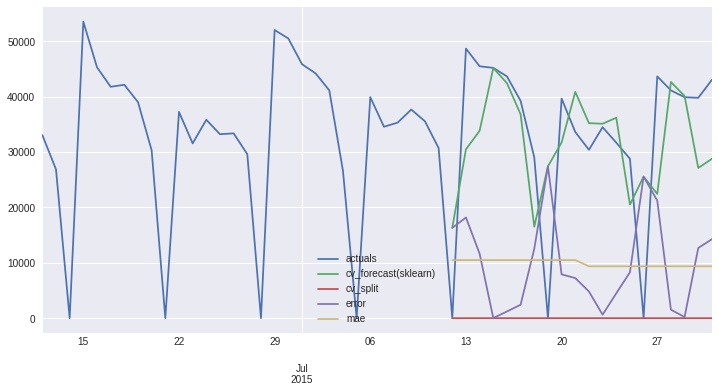
Data behind plots
Ready to be plotted or adjusted to your needs
[13]:
result.df_plot
[13]:
| actuals | cv_forecast(sklearn) | cv_split | error | cv_split_str | mae | |
|---|---|---|---|---|---|---|
| 2013-08-01 | 47527 | NaN | NaN | NaN | cv_split=nan, mae=nan | NaN |
| 2013-08-02 | 42200 | NaN | NaN | NaN | cv_split=nan, mae=nan | NaN |
| 2013-08-03 | 30370 | NaN | NaN | NaN | cv_split=nan, mae=nan | NaN |
| 2013-08-04 | 0 | NaN | NaN | NaN | cv_split=nan, mae=nan | NaN |
| 2013-08-05 | 42239 | NaN | NaN | NaN | cv_split=nan, mae=nan | NaN |
| ... | ... | ... | ... | ... | ... | ... |
| 2015-07-27 | 43671 | 22441.52 | 1 | 21229.48 | cv_split=1, mae=9370.22 | 9370.219 |
| 2015-07-28 | 41142 | 42666.69 | 1 | 1524.69 | cv_split=1, mae=9370.22 | 9370.219 |
| 2015-07-29 | 39906 | 40116.97 | 1 | 210.97 | cv_split=1, mae=9370.22 | 9370.219 |
| 2015-07-30 | 39800 | 27123.95 | 1 | 12676.05 | cv_split=1, mae=9370.22 | 9370.219 |
| 2015-07-31 | 43052 | 28785.73 | 1 | 14266.27 | cv_split=1, mae=9370.22 | 9370.219 |
730 rows × 6 columns
[14]:
result.df_plot.tail(50).plot();
[14]:
<AxesSubplot:>
[15]:
result
[15]:
ModelSelectorResult
-------------------
  best_model_name: sklearn
  frequency: D
  horizon: 10

  country_code_column: None

  partition: {'no_partition_label': ''}
  partition_hash: fb452abd91f5c3bcb8afa4162c6452c2

  df_plot: DataFrame (730, 6) suited for plotting cv results with .plot()
  X_train: DataFrame (730, 0) with training feature values
  y_train: DataFrame (730,) with training target values
  cv_results: DataFrame (2, 11) with gridsearch cv info
  best_model_cv_results: Series with gridsearch cv info
  cv_data: DataFrame (20, 4) with models predictions, split and true target values
  best_model_cv_data: DataFrame (20, 3) with model predictions, split and true target values

  model_reprs: Dict of model_hash and model_reprs
  best_model_hash: 53ec261970542c03a3b0a54fc6af214d
  best_model: Pipeline(memory=None,
         steps=[('exog_passthrough', 'passthrough'), ('holiday', 'passthrough'),
                ('model',
                 SklearnWrapper(bootstrap=True, ccp_alpha=0.0,
                                clip_predictions_lower=None,
                                clip_predictions_upper=None, criterion='mse',
                                fit_params=None, hcb_verbose=False, lags=3,
                                max_depth=None, max_features='auto',
                                max_leaf_nodes=None, max_samples=None,
                                min_impurity_decrease=0.0,
                                min_impurity_split=None, min_samples_leaf=1,
                                min_samples_split=2,
                                min_weight_fraction_leaf=0.0, n_estimators=100,
                                n_jobs=None, name='sklearn', oob_score=False,
                                optimize_for_horizon=False, random_state=42,
                                verbose=0, warm_start=False))],
         verbose=False)
-------------------
Best Model Metadata
That can help to filter for example cv_data or to get a glimpse on which parameters the best model has
[16]:
result.best_model_hash
[16]:
'53ec261970542c03a3b0a54fc6af214d'
[17]:
result.best_model_name
[17]:
'sklearn'
[18]:
result.best_model_repr
[18]:
"Pipeline(memory=None,steps=[('exog_passthrough','passthrough'),('holiday','passthrough'),('model',SklearnWrapper(bootstrap=True,ccp_alpha=0.0,clip_predictions_lower=None,clip_predictions_upper=None,criterion='mse',fit_params=None,hcb_verbose=False,lags=3,max_depth=None,max_features='auto',max_leaf_nodes=None,max_samples=None,min_impurity_decrease=0.0,min_impurity_split=None,min_samples_leaf=1,min_samples_split=2,min_weight_fraction_leaf=0.0,n_estimators=100,n_jobs=None,name='sklearn',oob_score=False,optimize_for_horizon=False,random_state=42,verbose=0,warm_start=False))],verbose=False)"
CV Results
Get information about how our model behaved in cross validation
[19]:
result.best_model_cv_results['mean_fit_time']
[19]:
0.0009076595306396484
Or how all the models behaved
[20]:
result.cv_results.sort_values('rank_test_score').head()
[20]:
| mean_fit_time | std_fit_time | mean_score_time | std_score_time | param_model | params | split0_test_score | split1_test_score | mean_test_score | std_test_score | rank_test_score | |
|---|---|---|---|---|---|---|---|---|---|---|---|
| 1 | 0.000908 | 0.000003 | 0.199280 | 0.001475 | SklearnWrapper(bootstrap=True, ccp_alpha=0.0, ... | {'model': SklearnWrapper(bootstrap=True, ccp_a... | -10491.576000 | -9370.219000 | -9930.89750 | 560.678500 | 1 |
| 0 | 0.001297 | 0.000441 | 0.019724 | 0.001840 | SklearnWrapper(clip_predictions_lower=None, cl... | {'model': SklearnWrapper(clip_predictions_lowe... | -12522.584395 | -8074.404344 | -10298.49437 | 2224.090025 | 2 |
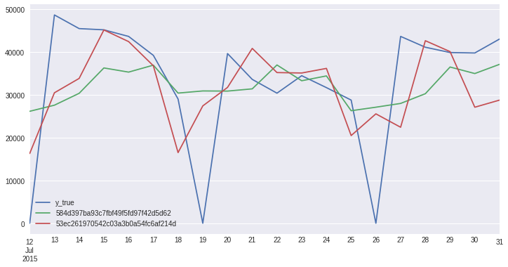
CV Data
Access predictions made during cross validation with possible cv splits and true target values
[21]:
result.cv_data.head()
[21]:
| split | y_true | 584d397ba93c7fbf49f5fd97f42d5d62 | 53ec261970542c03a3b0a54fc6af214d | |
|---|---|---|---|---|
| 2015-07-12 | 0 | 0.0 | 26171.429013 | 16311.14 |
| 2015-07-13 | 0 | 48687.0 | 27599.262145 | 30500.02 |
| 2015-07-14 | 0 | 45498.0 | 30372.219206 | 33853.97 |
| 2015-07-15 | 0 | 45209.0 | 36301.509820 | 45178.86 |
| 2015-07-16 | 0 | 43669.0 | 35328.104719 | 42460.11 |
[22]:
result.cv_data.drop(['split'], axis=1).plot();
[22]:
<AxesSubplot:>
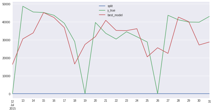
[23]:
result.best_model_cv_data.head()
[23]:
| split | y_true | best_model | |
|---|---|---|---|
| 2015-07-12 | 0 | 0.0 | 16311.14 |
| 2015-07-13 | 0 | 48687.0 | 30500.02 |
| 2015-07-14 | 0 | 45498.0 | 33853.97 |
| 2015-07-15 | 0 | 45209.0 | 45178.86 |
| 2015-07-16 | 0 | 43669.0 | 42460.11 |
[24]:
result.best_model_cv_data.plot();
[24]:
<AxesSubplot:>
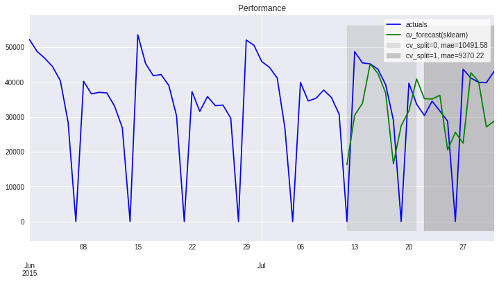
Plotting Functions
With **plot_params that you can pass depending on your plotting backend
[25]:
result.plot_result(plot_from='2015-06', title='Performance', color=['blue','green']);
[25]:
<AxesSubplot:title={'center':'Performance'}>
[26]:
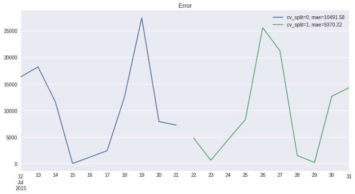
result.plot_error(title='Error');
[26]:
cv_split_str
cv_split=0, mae=10491.58    AxesSubplot(0.125,0.125;0.775x0.755)
cv_split=1, mae=9370.22     AxesSubplot(0.125,0.125;0.775x0.755)
Name: error, dtype: object
Convenient Persist Method
[27]:
result.persist?